Insights · CASE / 001 · Case study

Detecting under-performance in a solar array with a calibrated physical model

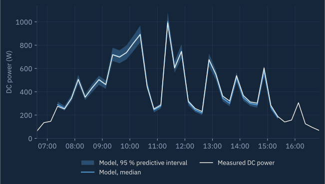
A year of measured output from a 1 kW heterojunction silicon array, compared interval by interval with a Bayesian-calibrated physical model. Faults are flagged only when they fall outside the model's own predictive uncertainty.

11 October 2026 · Model calibration · Anomaly detection · Uncertainty quantification

01 · ProblemIs the array under-performing, or is it just the weather?

A solar array's output changes all the time with sunlight and temperature. A fall in power can mean a fault (a failed inverter, snow, soiling, a broken string) or simply a cloud. A fixed threshold on power cannot tell these apart. The question is whether the measured output is consistent with what the physics predicts for the conditions actually observed, given the uncertainty of that prediction.

02 · Physical systemA 1 kW array at NREL, Golden, Colorado

Five 200 W heterojunction silicon modules (Sanyo HIP-200BA3), fixed at a tilt of 40° facing south, at an elevation of about 1,800 m. The array has its own plane-of-array irradiance sensor and a module-temperature sensor, which is what makes a physics-based comparison possible.

03 · DataOne year of public measurements

The National Renewable Energy Laboratory publishes minute-resolution data for this array (PVDAQ system 4) on the Open Energy Data Initiative. All of 2012 was used: DC power, plane-of-array irradiance $G$ and module temperature $T$ , averaged to 15-minute intervals. Intervals were kept when $G > 200 W m^{- 2}$ , the angle of incidence was below 75° and at least 12 of 15 minutes were present: 11,177 intervals on 361 days.

04 · ModelIrradiance, temperature and angle of incidence

DC power is proportional to irradiance, falls linearly as the cells warm, and loses a little more at oblique incidence because more light is reflected from the glass:

P = P_{ref} \frac{G}{1000} [1 + γ (T - 25^{\circ} C)] [1 - b_{0} (\frac{1}{cos θ} - 1)]

Here $P_{ref}$ is the output at 1000 W m⁻² and 25 °C, $γ$ the temperature coefficient, $b_{0}$ the incidence-angle coefficient and $θ$ the angle between the sun and the array normal, computed from the timestamp, location and array orientation. Each parameter has a physical meaning, so prior knowledge about it can be used.

05 · MethodBayesian calibration on two months, prediction on ten

The model was calibrated only on 1 March to 30 April, then used to predict every other interval of the year, which it had never seen. Priors encode what is known before looking at the data: $γ \sim N (- 0.30, 0.1 0^{2}) % /^{\circ} C$ , a typical value for heterojunction modules, and $b_{0} \sim N (0.05, 0.0 2^{2})$ , typical for glass-covered modules; $P_{ref}$ is left free. The residuals were modelled with a Student- $t$ distribution (4 degrees of freedom), so that the occasional bad interval in the calibration window does not drag the parameters.

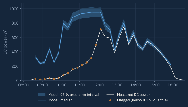
An interval is flagged when the measured power falls below the 0.1 % quantile of the posterior predictive distribution, which combines parameter uncertainty with the residual scatter. Days are compared on energy: measured against the predictive distribution of the day's total.

06 · ComputationMarkov chain Monte Carlo

The posterior was sampled with a random-walk Metropolis algorithm (60,000 iterations, 15,000 discarded as burn-in), and 2,000 posterior draws were propagated to every interval to form predictive distributions. The analysis is under 300 lines of Python (NumPy and Matplotlib) and runs in about ten seconds on a laptop.

07 · ResultThe model follows the weather; faults stand out

Parameter	Posterior mean [95 % interval]
Output at reference conditions, $P_{ref}$	918.5 [916.0, 921.0] W
Temperature coefficient, $γ$	-0.299 [-0.317, -0.283] %/°C
Incidence-angle coefficient, $b_{0}$	0.043 [0.038, 0.048]
Residual scale, $σ$	24.3 [23.3, 25.4] W

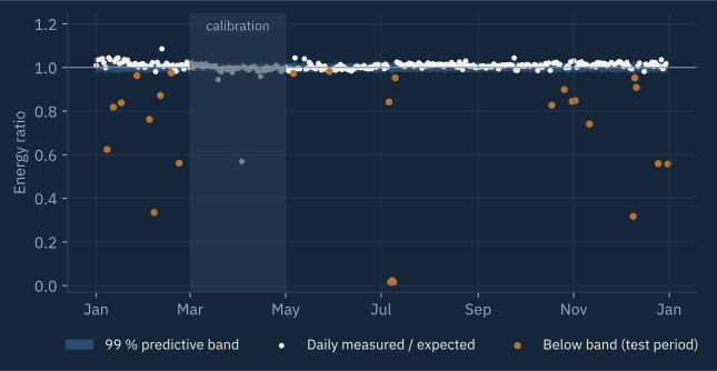
On a cloudy day, measured power rises and falls sharply many times and stays inside the model's narrow predictive band throughout. — FIG 1A cloudy day. Output swings between 200 W and 1,000 W as clouds pass. The model, driven by the measured irradiance and temperature, follows every change; no interval is flagged.

Daily ratio of measured to expected energy through 2012: most days sit near 1.0; a few fall well below the band, mostly in winter and in early July. — FIG 2The whole year, day by day. Measured energy divided by the model's median expectation. The shaded band is the 99 % predictive band for each day. Copper points are test-period days below it.

26 test-period days fall below their 99 % band. 5 of them produced less than half the expected energy:

Day	Measured (kWh)	Expected (kWh)	Mean air temperature
7 Feb 2012	0.35	1.04	-5.2 °C
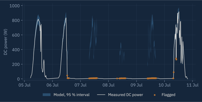
7 Jul 2012	0.06	3.85	22.1 °C
8 Jul 2012	0.03	1.35	19.6 °C
9 Jul 2012	0.06	3.70	21.6 °C
9 Dec 2012	0.37	1.18	-6.8 °C

Six days in July 2012: normal output on 5 July, output falling to zero on the afternoon of 6 July, near-zero output through 9 July despite sunlight, and recovery on 10 July. — FIG 3An outage. From the afternoon of 6 July to the morning of 10 July the array produced almost nothing while the irradiance sensor recorded normal summer sunlight. Every daylight interval is flagged.

On 25 December 2012, measured output is far below the model's band in the morning and rises to meet it shortly after midday. — FIG 4A winter morning. On 25 December, with a mean air temperature of −9.5 °C, output stays far below the prediction until shortly after noon and then rejoins the band. The pattern is consistent with snow or frost clearing from the modules.

08 · UncertaintyHow far to trust the bands

On the calibration window, 94.9 % of intervals fall inside the 95 % predictive interval, as they should. On the ten unseen months the figure is 90.2 %: the bands are slightly too narrow away from the calibration season. This is expected, because two spring months cannot capture every seasonal effect, and it is why flags use the far tail (0.1 %) rather than the 95 % edge.

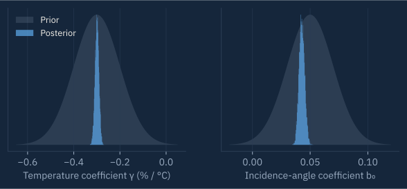
Two panels: the posterior distribution of the temperature coefficient and of the incidence-angle coefficient, each much narrower than its prior. — FIG 5Prior knowledge updated by data. Grey: priors from module physics. Blue: posteriors after calibration. The data narrow both coefficients by roughly a factor of ten.

The posterior temperature coefficient, -0.30 %/°C, is close to the prior centre and to typical published values for heterojunction modules. The incidence-angle coefficient, 0.043, is close to the value usually assumed for glass. Both are physically plausible, which is a check on the model, not just on the fit.

09 · InterpretationWhat the flags mean

Out of 9,067 unseen intervals, 332 (3.7 %) were flagged, and most belong to a handful of events. The July event is an outage: sunlight was present and output was essentially zero for three and a half days. The large winter shortfalls all occur on days with sub-freezing air temperatures, consistent with snow cover; on 25 December the output visibly recovers once it clears. A monitoring system built this way would raise a few clear alarms per year instead of one every cloudy afternoon.

10 · LimitationsWhat this study does not show

The cause of each event is inferred, not observed. There are no maintenance logs or camera images; "snow" is a plausible explanation consistent with the temperatures, not a confirmed one.
A residual afternoon bias remains: measured output exceeds the model by up to 5.7 % between 15:00 and 17:00. Likely causes are thermal lag of the back-of-module temperature sensor and differences between the sensor's and the modules' angular response. The model does not include them.
Daily energy bands treat interval errors as independent. Real errors are correlated within a day, so the daily bands are too narrow; small daily shortfalls should not be read as faults.
The method needs on-site irradiance and module temperature. Where only satellite irradiance is available, prediction uncertainty is larger and fewer faults can be detected.
One array and one year. The approach transfers to other systems, but each needs its own calibration and validation.

ReproduceCode and data

The data are fetched from the public PVDAQ archive with analysis/case001_pv_anomaly/fetch_data.py; analysis.py performs the calibration, prediction and figures, and writes every number on this page to results.json. The random seed is fixed.

References

National Renewable Energy Laboratory. Photovoltaic Data Acquisition (PVDAQ) public dataset, system 4, via the Open Energy Data Initiative data lake, s3://oedi-data-lake/pvdaq/.
J. W. Spencer (1971). Fourier series representation of the position of the sun. Search 2(5), 172. (Solar position used for the angle of incidence.)
R. F. Souka and H. H. Safwat (1966). Determination of the optimum orientations for the double-exposure, flat-plate collector and its reflectors. Solar Energy 10, 170–174. (Origin of the incidence-angle modifier.)
A. Gelman, J. B. Carlin, H. S. Stern, D. B. Dunson, A. Vehtari and D. B. Rubin (2013). Bayesian Data Analysis, 3rd ed. CRC Press.