Insights · NOTE / 001 · Technical note

Reporting a result with its uncertainty

Why a measured value without an interval is incomplete, and how to propagate input uncertainty through a model, using a pendulum measurement of g as the worked example.

11 October 2026 · Uncertainty quantification

A number without an interval

"g = 9.808 m/s²" looks precise. It is not, and the four decimals say nothing about whether it agrees with the accepted 9.81 m/s². A measured or computed result becomes usable only when it carries an interval, and when the input that dominates that interval is known.

The measurement

A pendulum of length $L = 0.7500 \pm 0.0015 m$ is timed over 20 oscillations: $20 T = 34.75 \pm 0.12 s$ . The uncertainty in the timing is dominated by reaction time at start and stop. These values are a worked example chosen to be typical of a careful bench measurement. With the small-angle model,

g = \frac{4 π ^{2} L}{T ^{2}} .

Linear propagation

For small, independent uncertainties, relative uncertainties add in quadrature, weighted by the power each quantity carries in the formula:

\frac{σ _{g}}{g} = (\frac{σ _{L}}{L})^{2} + (2 \frac{σ _{T}}{T})^{2} .

This gives $σ_{g} = 0.071 m/ s^{2}$ . The period enters squared, so its relative uncertainty counts twice: timing contributes 92 % of the variance, length only 8 %.

Monte Carlo propagation

Linearisation can fail when uncertainties are large or the model is strongly nonlinear. The general method is to sample the inputs from their distributions, push every sample through the model and look at the distribution of results. With 200,000 samples:

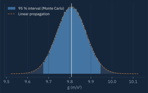
Histogram of g from 200,000 Monte Carlo samples with the central 95 % interval shaded; the linear-propagation normal curve lies on top of it. — FIG 1Distribution of g. Shaded: central 95 % of the Monte Carlo samples. Dashed: the normal distribution from linear propagation. Here the two agree, which confirms that the linear result can be used.

Method	g (m/s²)	Standard uncertainty	95 % interval
Linear propagation	9.808	0.071	9.67 – 9.95
Monte Carlo	9.808	0.070	9.67 – 9.95

How to report it

Result

$g = 9.81 \pm 0.07 m/ s^{2}$ (standard uncertainty), 95 % interval 9.67 to 9.95 m/s². Timing dominates (92 % of the variance).

Three things make this a complete result. The value is rounded to match its uncertainty. The interval is stated with its meaning (standard uncertainty or 95 %). And the dominant source is named, which tells the reader what to improve: timing 50 oscillations instead of 20 would do far more than a better ruler.

The accepted value, 9.81 m/s², lies inside the interval. Without the interval, that comparison could not be made at all.

Beyond the pendulum

The same steps apply to any model: list the uncertain inputs, assign each a distribution, propagate, and report the result with its interval and its dominant source. In larger problems the inputs are model parameters inferred from data, as in CASE / 001, and the model is a simulation, but the logic does not change. The model itself is also an approximation: at large amplitudes the small-angle formula used here is biased, an error no amount of careful timing will reveal.

References

JCGM 100:2008. Evaluation of measurement data: Guide to the expression of uncertainty in measurement (GUM).
JCGM 101:2008. Supplement 1 to the GUM: Propagation of distributions using a Monte Carlo method.

Code: analysis/methods/figures.py (function uq_pendulum).